3D - Subaerial and Submarine solid slides

The two-dimensional domain [-2, 6] x [-1.85, 1.85] is discretized with Ax = 0.02 Tit and the number of layers was set up to 3. Similar results were observed if more layers are considered. The final time is 4 s, CFL number was set to 0.9 and g =. 9.81. The same boundary conditions as in the previous case were imposed. In order to capture turbulent processes, as in benchmark 1, the complete Navier-Stokes viscous stress tensor is used with the same subgrid model and coefficients. Figures 6 and 7 show the numerical results obtained for the subaerial test case, first presenting the comparison for the wave gauges (Fig. 6) and the for the runup gauges (Fig. 7) . The same comparison can be found in Figures 8 and 9 for the submerged test case. 

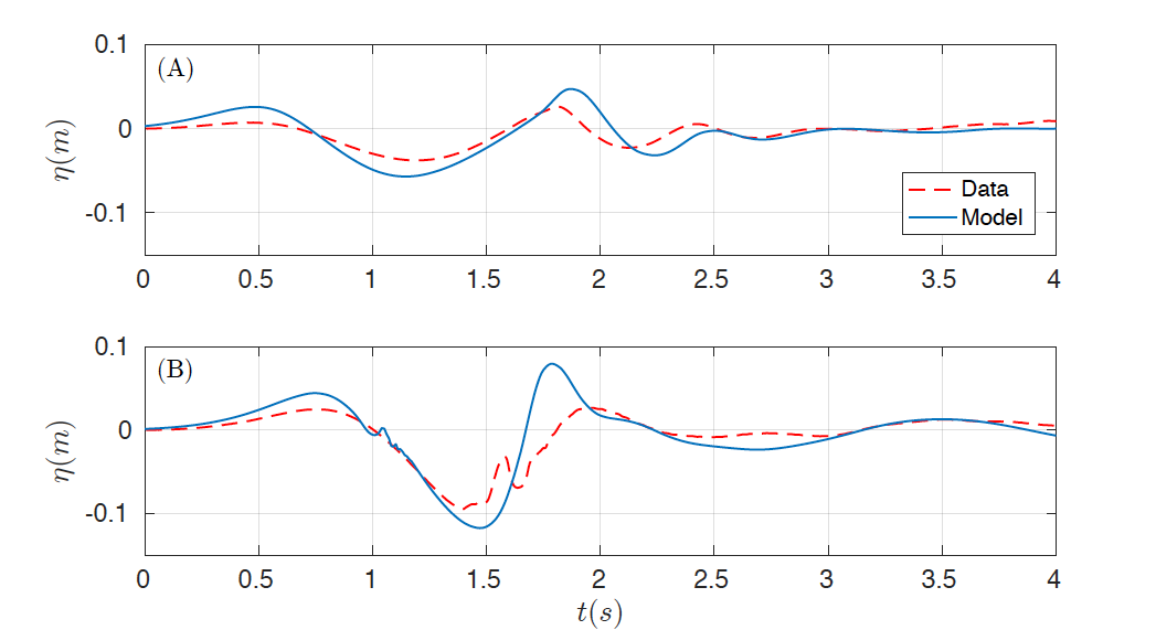
Figure 6. Comparison of data time series (red) and numerical (blue) at wave gauges (A) WG1 and (B) WG2 for the subaerial case.

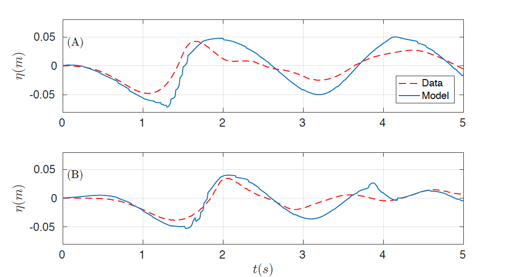
Figure 7. Comparison of data runup time series (red) and numerical (blue) at runup gauges (A) RG2 and (B) RG3 for the subaerial case.

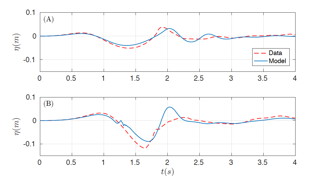
Figure 8. Comparison of data time series (red) and numerical (blue) at wave gauges (A)  WG1  and (B)  WG2 for the submerged case.

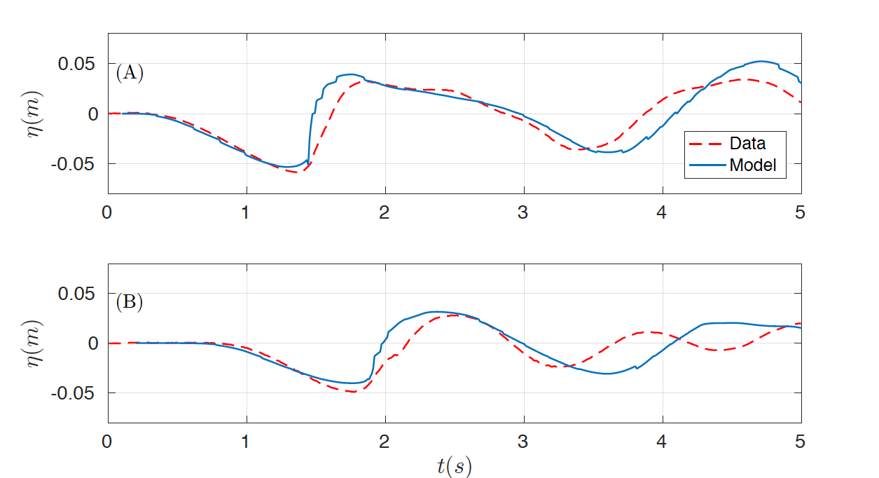
Figure 9. Comparison of data runup time series (red) and numerical (blue) at runup gauges (A) RG2 and (B) RG3 for the submerged case.