Two-dimensional submarine solid block

In this benchmark two items remain undetermined: they are the initialization of the numerical experiment and the second one is how and where and how the moving solid block must stop. 

The one-dimensional domain [-1, 10] is discretized with Ax = 0.02 m and the number of layers was set up to 3. Similar results were obtained with more layers. The simulated time was 4 s. CFL was set to 0.9 and g = 9.81. Outflow boundary conditions are used. In order to capture turbulent processes, following Ma et al (2012), the complete Navier-Stokes viscous stress tensor is used, where the turbulent kinematic viscosity is estimated by. the Smagorinsky subgrid model, with Cs = 0.2 (Smagorinsky turbulent coefficient) and k, = 0.01 (bottom roughness height). 

First, we would like to stress that we found a bit confusing geometry definition for this benchmark problem, mainly due to the sometimes unclear use of dimension and dimensionless variables, not always consistent with the non-tilde vs tilde notation, respectively. In our presentation at the workshop, we stressed the mismatch we found between provided data and figures in the benchmark description: we were not able to reproduce, with the given data, the figures provided in the document describing the benchmark. To illustrate this fact, we presented the numerical results obtained with the Multilayer-HySEA model that has been adimensionalized in time dividing by to = 1.677 and compared them with the measured data, first adimensionalized using the same value (as should be coherent, but the resulting figure does not agree with the figures provided in the benchmark description) and then using the value T = to + ti (with ti the initialization time appearing in the benchmark problem description) to adimensionalize. Here we have compared the numerical results with the lab data adimensionalized using the former value for T.

In Figure 3 comparison of filtered lab measured data with numerical results are presented. 

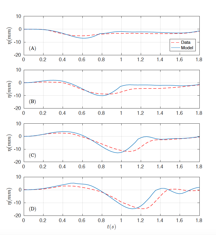
Figure 3. Comparison of filtered data time series (red) and numerical (blue) at wave gauges (A) g1 , (B) g2 , (C) , and (D) g3.