Benchmark Description
The goal of this Benchmark Problem is to compare computed model results with field measurements gathered after the 12 July 1993 Hokkaido-Nansei- Oki tsunami (also commonly referred to as the Okushiri tsunami).
Problem Set-up
The main items describing the setup of the numerical problem are:
- Friction. Manning coefficient 0.03.
- Boundary conditions. Non-reflective boundary conditions at open sea, at coastal areas inundation is computed.
- Computational domain. A nested mesh technique is used with four levels (i.e., the global mesh with three levels of refinement, see Figure BP6.1 and BP6.2).
- Global mesh covering in lon/lat [138.504, 140.552] x [41.5017,43.2984],
- Number of cells: 1,152 x 1,011 = 1,164,672.
- Resolution: 6.4 arc-sec (approx 192 m)Level 1. Spatial coverage [139.39,139.664] x [41.9963,42.2702],
- Level 1. Spatial coverage [139.39,139.664] x [41.9963,42.2702],
- Refinement ratio: 4,
- Number of cells: 616 x 616 = 379,456
- Resolution: 1.6 arc-sec (approx 40 m)
- Level 2. Refinement ratio: 4. Resolution: 0.4 arc-sec (approx 12 m)
- Submesh 1. Large area around Monai.
- Spatial coverage [139.434,139,499] x [42.0315,42.0724],
- Number of cells: 584 x 368 = 214,912
- Submesh 2. Aonae cape and Hamatsumae region
- Spatial coverage [139.411, 139.433] x [42.0782, 42.1455],
- Number of cells: 196 x 604 = 118,384
- Submesh 1. Large area around Monai.
- Level 3 (Monai region). Spatial coverage [139.414, 139.426] x [42.0947, 42.1033],
- Refinement ratio: 16,
- Number of cells: 1,744 x 1,248 = 2,216,448
- Resolution: 0.025 arc-sec (approx 0.75 m)
- Global mesh covering in lon/lat [138.504, 140.552] x [41.5017,43.2984],
-
Initial condition. Generated by DCRC (Disaster Control Research Center), Japan. Hipocenter depth 37 km at 139.32º E and 42.76º N, Mw 7.8 (Takahashi, 1996). In Fig. BP9.2 (source model DCRC 17a).
-
Topobatymetric data. Kansai University
-
CFL. 0.9
-
Model used. Tsunami-HySEA WAF
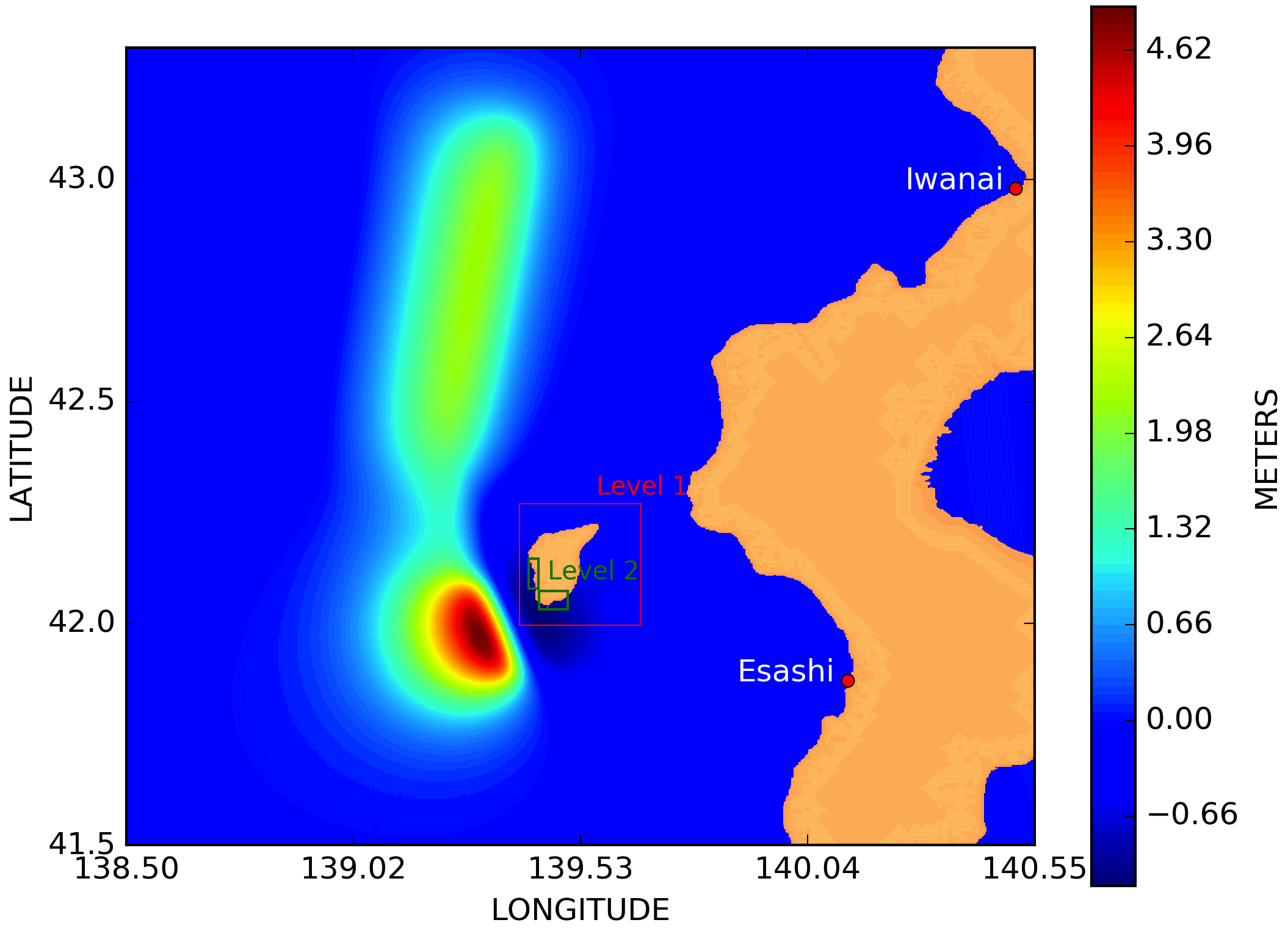
Figure BP9.1. Computational domain considered (level 0), showing the initial condition for Benchmark problem #9. Nested meshes level 1 and level 2 (the latter composed of two submeshes) are also depicted.
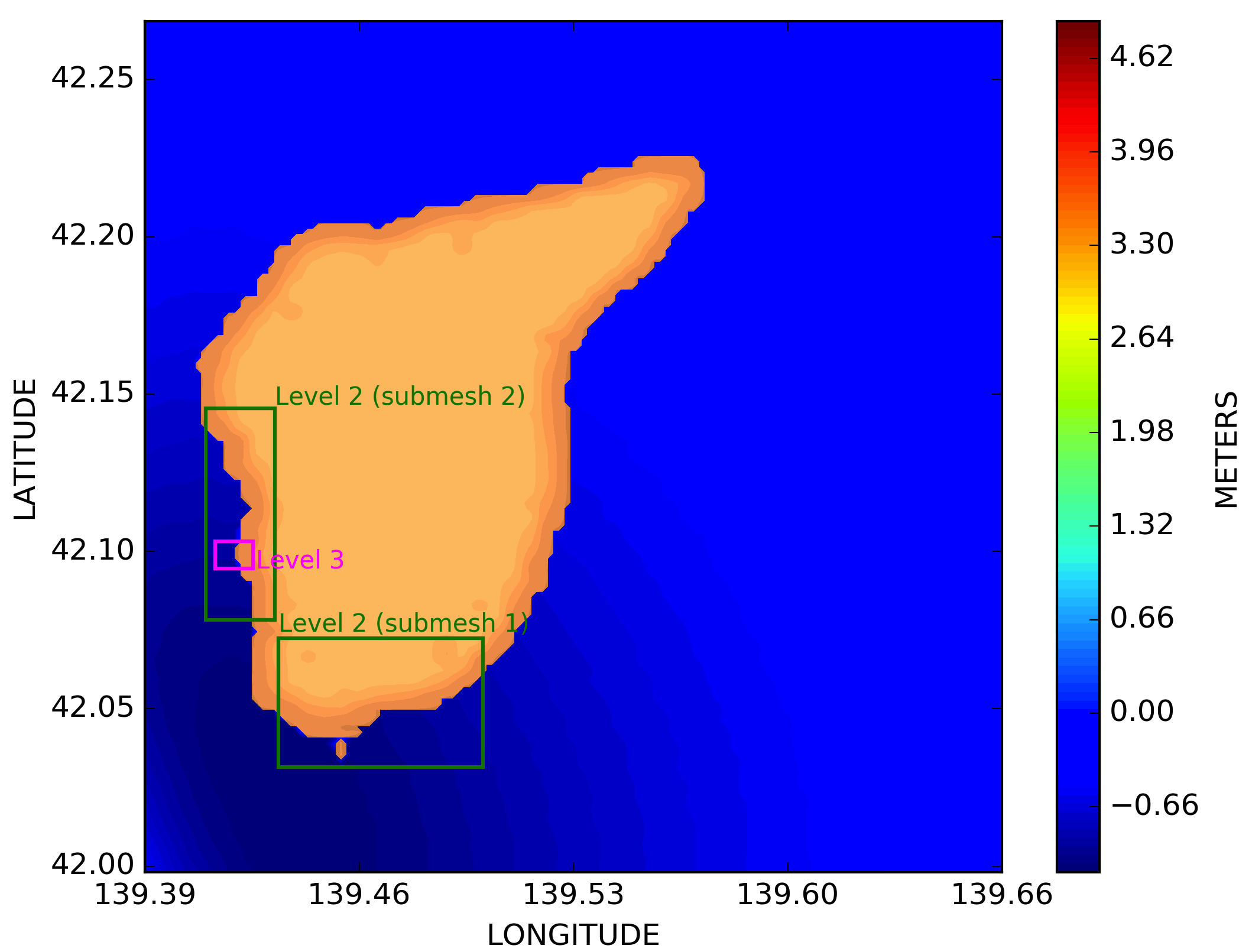
Figure BP9.2. Level 1 nested mesh computational domain containing the two level 2 submeshes, the region to the South including Aonae and Hamatsumae areas and the coastal region to the West containing Monai area, refined with one level 3 nested mesh around Monai Valley.
Tasks to be performed
- Compute runup around Aonae.
- Compute arrival of the first wave to Aonae.
- Show two waves at Aonae approximately 10 min apart; the first wave came from the west, the second wave came from the east.
- Compute water level at Iwanai and Esashi tide gauges.
- Maximum modeled runup distribution around Okushiri Island.
- Modeled runup height at Hamatsumae.
- Modeled runup height at a valley north of Monai.
Tasks to be performed
Task 1 Runup aroud Aonae
Figure BP9.3 shows the inundation level around Aonae peninsula. The figure includes 4-meter contours of bathymetry and topography. The contours allow to determine that the maximum runup height is below 12 m in the eastern part of the peninsula where the tsunami inundation is mainly produced by the second wave and where the topography is flatter producing, despite the lower runup, a further penetration. The opposite situation occurs in the western part of the peninsula: a higher runup ranging from 16 to 20 m, within a narrower strip, mainly flooded by the first wave arriving from the west. The southern part of the peninsula is inundated with a runup height of 16 meters and a large inundated area.
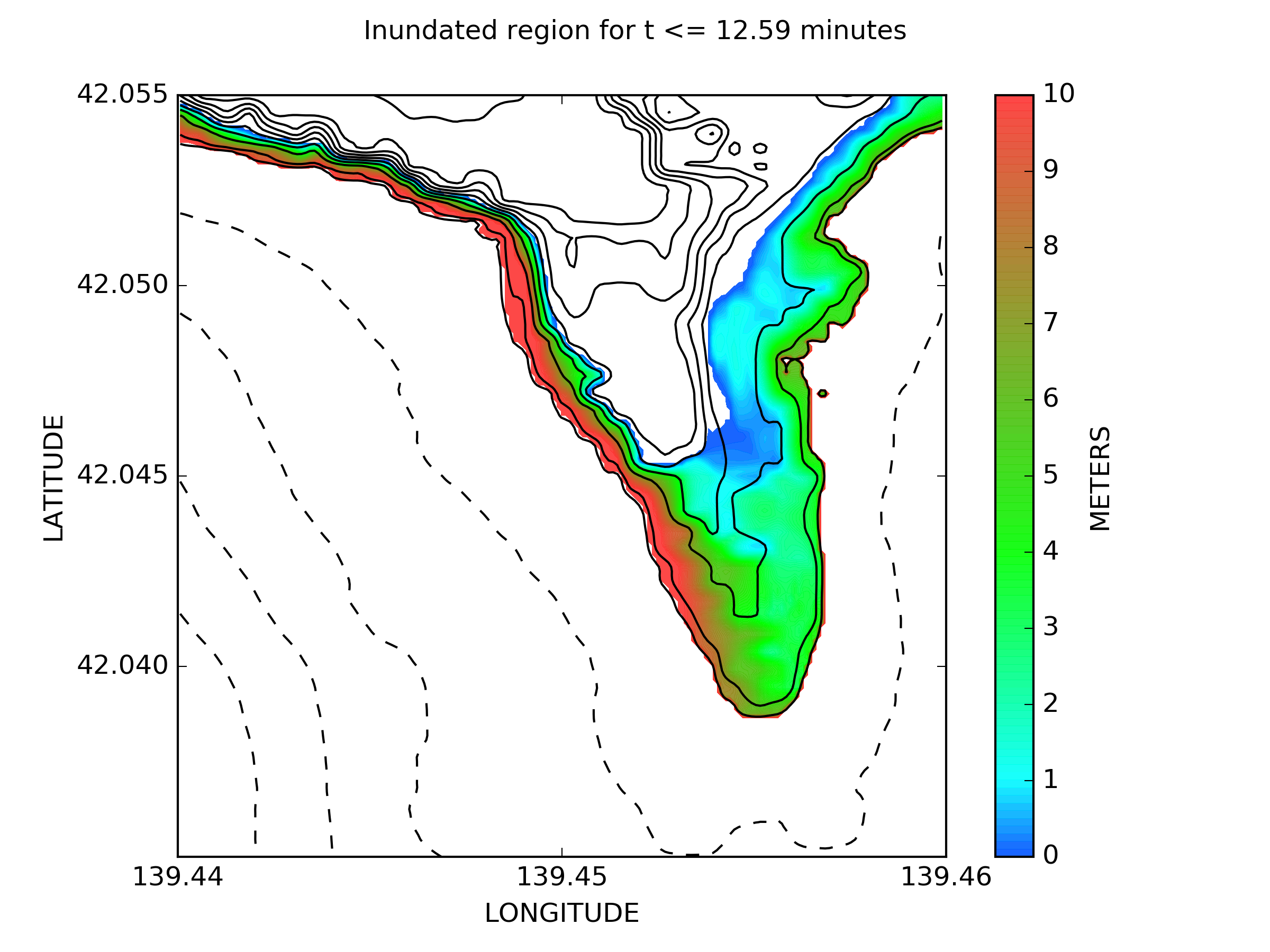
Figure BP9.3. Inundation map of the Aonae Peninsula. This is for t<12.59 min. The color map shows the maximum fluid depth over entire computation. 4-meter contours of bathymetry and topography are shown.
Tasks to be performed
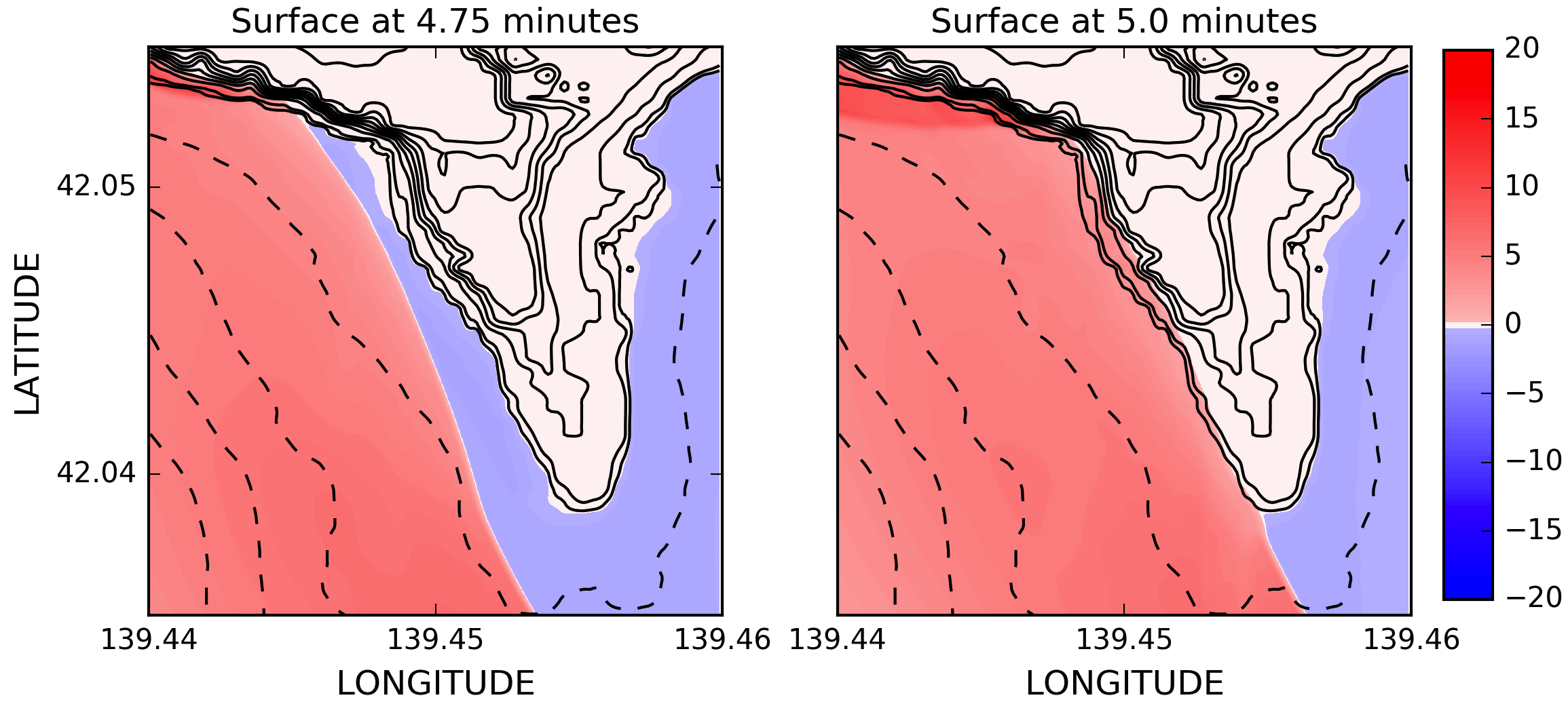
Task 2 First wave to Aoane
Figure BP9.4 shows the arrival of the first wave, coming from the west, to the Aonae peninsula at times t=4.75 min and t=5 min. From this figure we can conclude the time of arrival of this first wave to Aoane takes place at approximately t=5 min. Within 15 seconds the wave is close to reach the western coastline of the peninsula and at t=5 min it has already impacted, from north to south, along all the western seashore.
Tasks to be performed
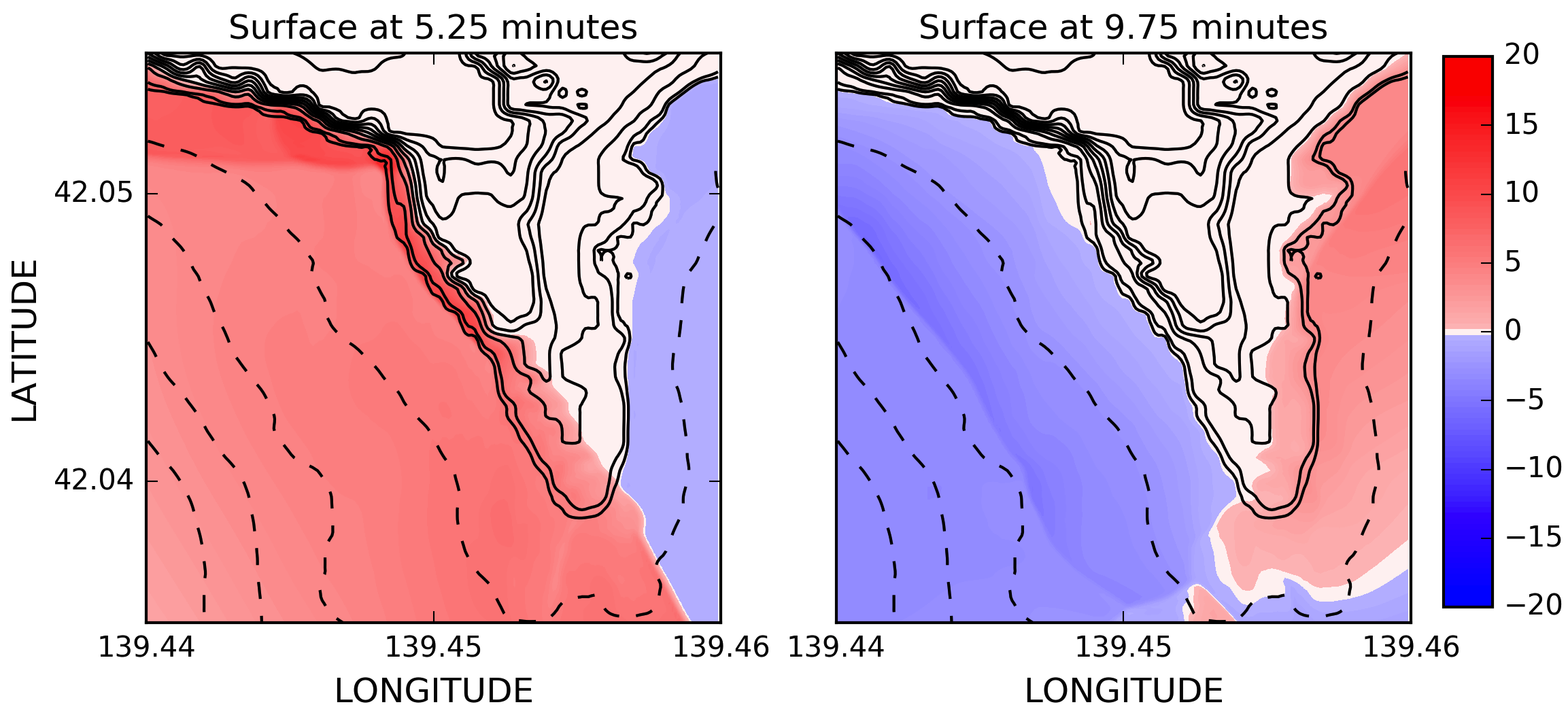
Task 3 Waves arriving to Aonae
Figure BP9.5 depicts two snapshots of the arrival of two tsunami waves to the Aonae peninsula. The first wave arrival, from the west, is seen at about t=5 minutes, as was shown in Figure BP9.4. The second major wave arrives from the east at about 9.5 minutes. Snapshots at time t=5.25 min and t= 9.75 min are presented in Figure BP9.5.
Tasks to be performed
Task 4 Tide gauges at Iwanai and Esashi
Figure BP9.6 shows the comparison between the computed and observed water levels at two tide stations located along the west coast of Hokkaido Island, Iwanai and Esashi. Besides, the maximum error in the maximum wave amplitude and the Normalized root mean square deviation (NRMSD) is depicted for both time series. The errors in the maximum amplitude, although high (36% and 41%) are analogous to the mean of the models collected in NTHMP (2012) report (36% and 43%, respectively). In this report, no values were given for the NRMSD.

Tasks to be performed
Task 5 Maximum runup around Okushiri
Figure BP9.7 shows a bar plot that compares model runup at 19 regions around Okushiri Island with measured data. In the NTHMP-provided script, runup error is evaluated by a comparison between computed and measured sets of minimal, maximal, and mean runup values in unspecified surroundings of prescribed reference points. We have searched for the set of observations used for each region to compute the minimal, maximal and mean values. For each of these observed values the closer or the two closer model values were considered for the computation of the minimum, maximum and the average in the given region. This was done in all cases, but in the regions with refined meshes, where all computed values were used. In Table BP9.1 the location of the points identifying these 19 regions are gathered and for each region the number of observations used to determine minimal, maximal and mean values are given in column #OBS. Finally, this table also presents Tsunami-HySEA runup error at each location compared with the mean of models in NTHMP (2012).
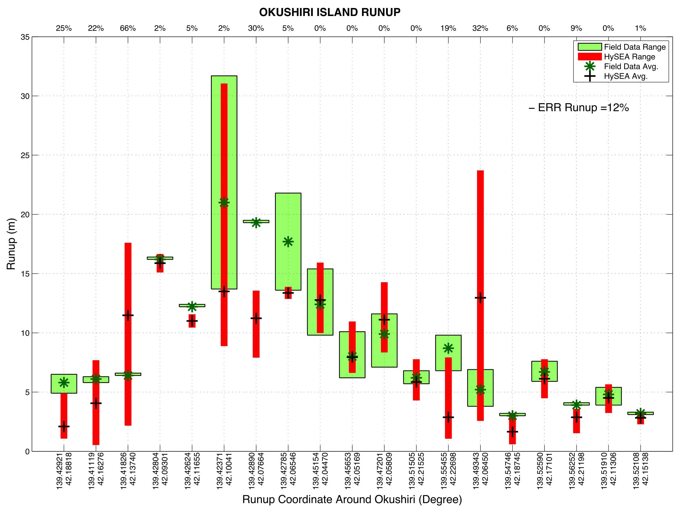
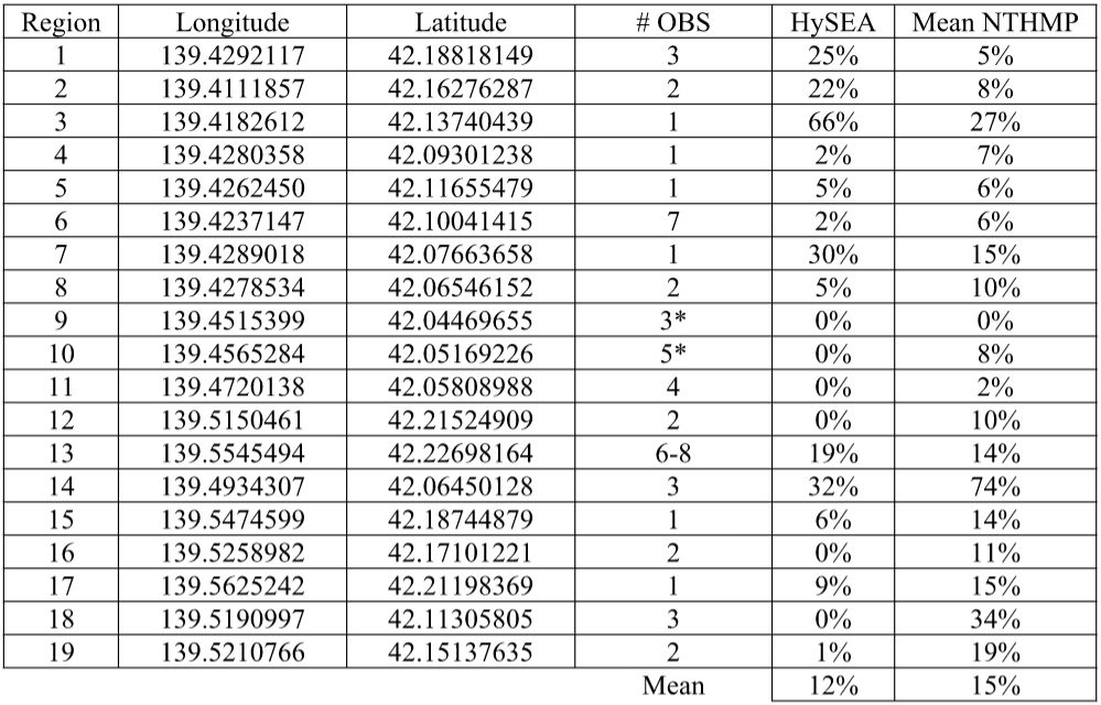
Table BP9.1. Tsunami-HySEA model relative error with respect to field measurement data for runup around Okushiri Island. Comparison with average error values for models in NTHMP (2102). #OBS gives the number of observations used to compute the error bars in Figure BP9.7 (*) when one observed value has been skipped. NTHMP data taken from Table 1-11 b in page 49.
Tasks to be performed
Task 6 Runup height at Hamatsumae
Figure BP9.8 shows the maximum inundation on the Hamatsumae region computed for [0,14] min. The color map shows the maximum fluid depth along the entire simulation. The figure also depicts 4-meter contours of bathymetry and topography. Maximum runups are between 8 and 16 meters, with increasing values from west to east.
Tasks to be performed
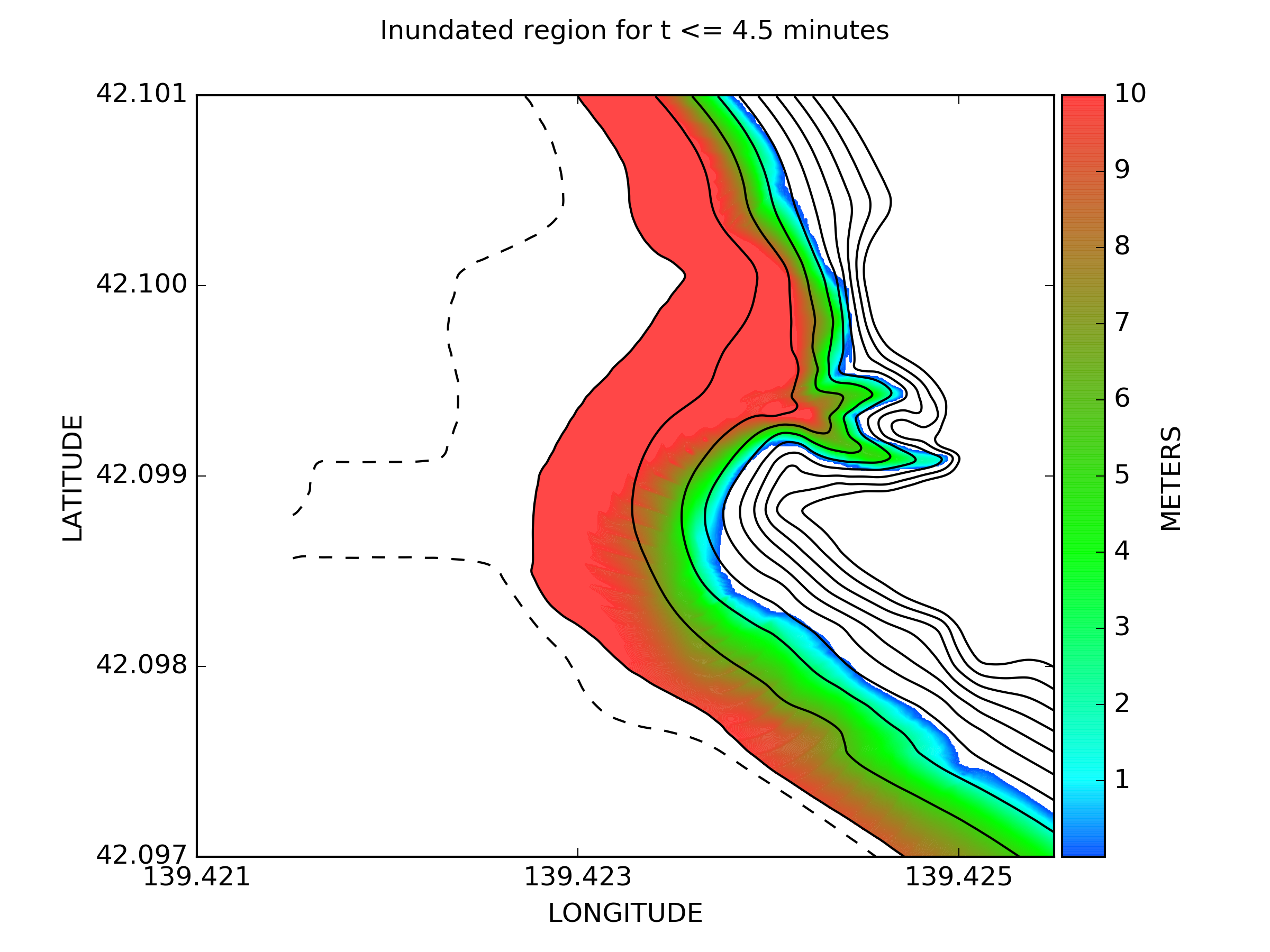
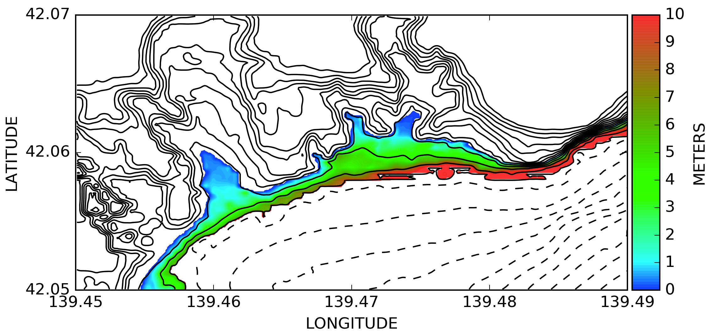
Task 7 Runup height at a valley north of Monai.
Figure BP9.9 shows the maximum inundation at a valley north of Monai, computed for [0,4.5] min. The color map shows the maximum fluid depth along the entire simulation. The 4-meter contours of topography allows to determine maximum runups that range between 8 and 12 meters to the south, around 16 to the north and up to the 31.753 meters of maximum computed runup, very close to the 31.7 meters observed value.