Benchmark Description
The goal of this benchmark problem is to compare computed model results with laboratory measurements obtained during a physical modeling experiment conducted at the Coastal and Hydraulic Laboratory, Engineering Research and Development Center of the U.S: Army Corps of Engineers (Briggs et al. 1995). The laboratory physical model was constructed as an idealized representation of Babi Island, in the Flores Sea, Indonesia, to compare with Babi Island runup measured shortly after the 12 December 1992 Flores Island tsunami (see Figure 1 below for a schematic picture).

Figure 1 Basin geometry and coordinate system. Solid lines represent approximate basin and wavemakers surfaces. Circles along walls and dashed lines represent wave absorbing material. Red dots represent gage locations for time series comparison. (Figure adapted from benchmark description).
Three cases (A, B, and C) were performed corresponding to three wavemaker paddle trajectories.
To accomplish this benchmark, it is suggested that, for
- CASE B: Water Depth, d = 32.0 cm, Target H = 0.10, Measured H = 0.096 (This case was formerly optional).
- CASE C: Water Depth, d = 32.0 cm, Target H = 0.20, Measured H = 0.181.
To perform the tasks described below.
The case A, that was formerly mandatory, now it is not included:
- CASE A: Water Depth, d = 32.0 cm, Target H = 0.05, Measured H = 0.045
In any case, we will include the three cases for all the tasks but for the splitting-colliding item.
Problem Set-up
The main items describing the numerical setup of the problem are:
- Friction. Manning coefficient is set to 0.015 for the non dispersive model and to 0.02 for the dispersive model.
- Computational domain. [-5,23]x[0,28] in meters.
- Boundary conditions. Open boundary conditions.
- Initial condition. The prescribed soliton centered at x=0 with the proposed correction for the initial velocity.
- Grid resolution. A spatial grid resolution of 5 cm is used for Case A and a 2 cm resolution grid for Cases B and C for the non-dispersive model. Dispersive model uses a 2cm resolution for the three cases.
- Time stepping. Variable time stepping based on a CFL condition.
- CFL. 0.9
- Version of the code. Tsunami-HySEA second order (non-dispersive) and second order dispersive codes have been used.
Tasks to be performed
Model simulations must be conducted to address the following objectives (for cases B and C):
- Demonstrate that two wave fronts split in front of the island and collide behind it;
- Compare computed water level with laboratory data at gauges 9, 16, and 22;
- Compare computed island runup with laboratory gage data.
Numerical Results
Note that, as we used the script MATLAB files and data provided by J. Horrillo, we decided to perform numerical experiments for all the three cases A, B, and C, and also to present water level at gauge 6, although not included as mandatory requirements. For this benchmark we have used Tsunami-HySEA non-dispersive and dispersive codes.
Tasks to be performed
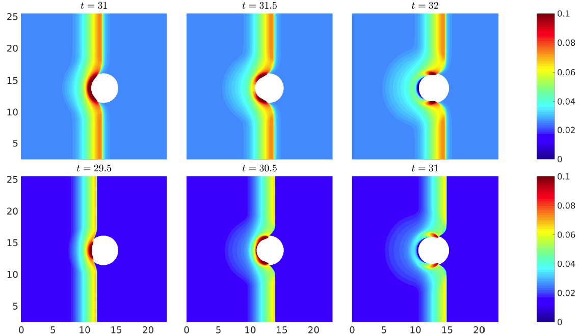
Task 1 Wave splitting and colliding
Figures BP6.1.a and b present snapshots at different times for case B and C, respectively, showing how two wave fronts split in front of the island (Task 1). For case B times t=31, 31.5, and 32 are shown and for case C times t=29.5, 30.5, and 31.
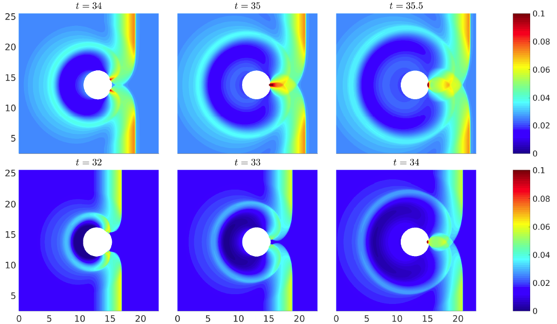
Figures BP6.1.c and d present snapshots at different times for case B and C, respectively, showing how two wave fronts, after splitting, collide behind the island (Task 1). For case B times t=34, 35, and 35.5 s are shown and for case C times t=32, 33, and 34 s.
Tasks to be performed
Task 2 Water level at gauges
In this section we present the comparison of the computed and measured water level at gauges 6, 9, 16, and 22 for the cases (A), (B), and (C), respectively. First the results for the non-dispersive model are presented, then the results for the dispersive code.
Figures BP6.2 (a, b, and c) present the comparison for water level at gauges 6, 9, 16, and 22 for the cases (A), (B), and (C) of the computed with Tsunami-HySEA non-dispersive model and measured data.
Figures BP6.2D (a, b, and c) present the comparison for water level at gauges 6, 9, 16, and 22 for the cases (A), (B), and (C) of the computed with Tsunami-HySEA dispersive model and measured data. Tables BP6.1 (a, b, and c) gather the sea level time series Tsunami-HySEA non- dispersive and dispersive models error with respect to laboratory experiment data for Case A, B, and C, respectively. Comparison with the mean value obtained for the 8 models performing this benchmark in NTHMP (2012) split into non-dispersive and dispersive models is also included.

Figure BP6.2.a Comparison between the computed and measured water level at gauges 6, 9, 16, and 22 for an incident solitary wave in the case A (H=0.045). Tsunami-HySEA non-dispersive model.
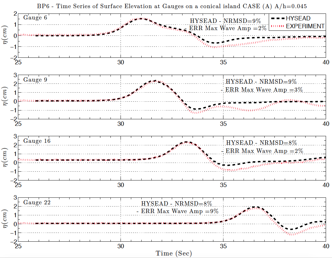
Figure BP6.2D.a Comparison between the computed and measured water level at gauges 6, 9, 16, and 22 for an incident solitary wave in the case A (H=0.045). Tsunami-HySEA dispersive model.
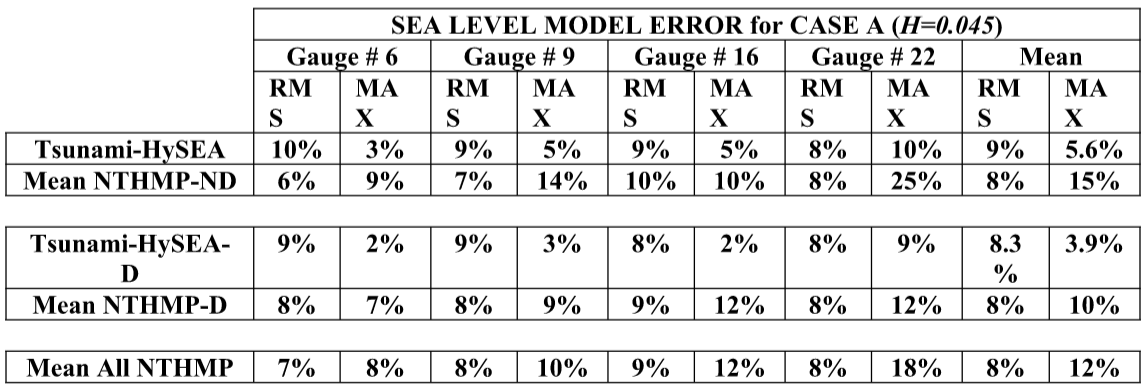
Table BP6.1.a Sea level time series Tsunami-HySEA model error with respect to laboratory experiment data for Case A (H=0.045). Comparison with the mean value obtained for the 8 models performing this benchmark in NTHMP (2012) separated among non-dispersive (Alaska, Geoclaw, and MOST) and dispersive models (ATFM, BOSZ, FUNWAVE, NEOWAVE, and SELFE), for a more precise comparison. RMS: Normalized Root Mean Square Deviation Error. MAX: Maximum runup relative error. The values for NTHMP models are taken from data in Table 1-9 a of NTHMP (2012).

Figure BP6.2.b Comparison between the computed and measured water level at gauges 6, 9, 16, and 22 for an incident solitary wave in the case B (H=0.096). Tsunami-HySEA non-dispersive model.

Figure BP6.2D.b Comparison between the computed and measured water level at gauges 6, 9, 16, and 22 for an incident solitary wave in the case B (H=0.096). Tsunami-HySEA dispersive model.
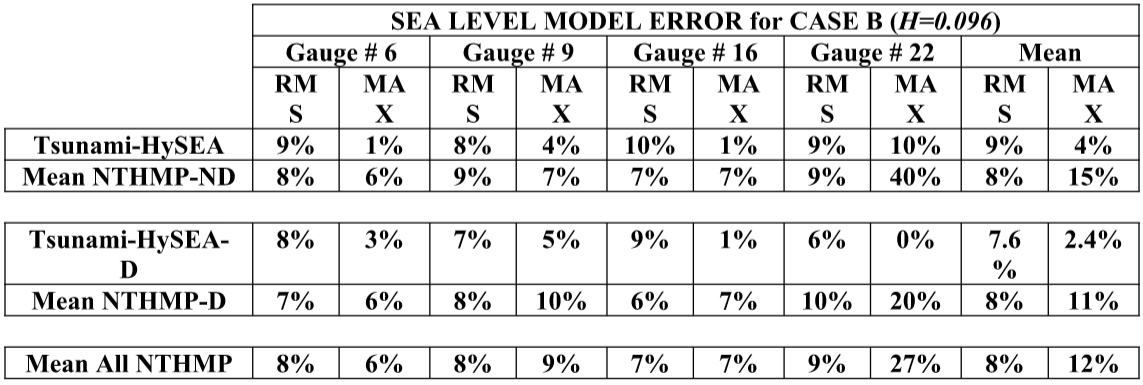
Table BP6.1.b Sea level time series Tsunami-HySEA model error with respect to laboratory experiment data for Case B (H=0.096). Comparison with the mean value obtained for the 8 models performing this benchmark in NTHMP (2012) separated among non-dispersive (Alaska, Geoclaw, and MOST) and dispersive models (ATFM, BOSZ, FUNWAVE, NEOWAVE, and SELFE), for a more precise comparison. RMS: Normalized Root Mean Square Deviation Error. MAX: Maximum runup relative error. The values for NTHMP models are taken from data in Table 1-9 b of NTHMP (2012).
Root Mean Square Deviation Error. MAX: Maximum runup relative error. The values for NTHMP models are taken from data in Table 1-9 b

Figure BP6.2.c Comparison between the computed and measured water level at gauges 6, 9, 16, and 22 for an incident solitary wave in the case C (H=0.181). Tsunami-HySEA non-dispersive model.
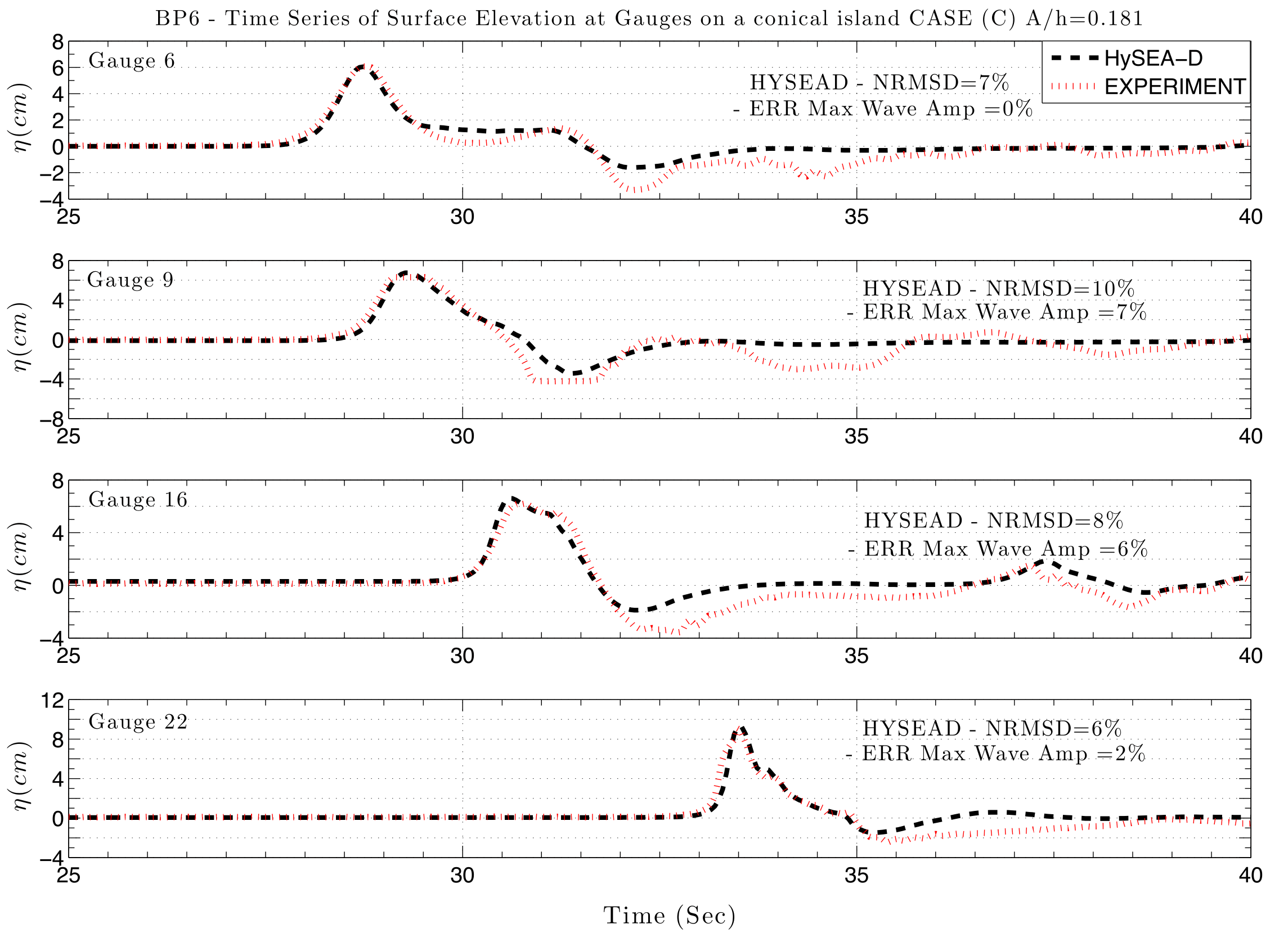
Figure BP6.2D.c Comparison between the computed and measured water level at gauges 6, 9, 16, and 22 for an incident solitary wave in the case C (H=0.181). Tsunami-HySEA dispersive model.
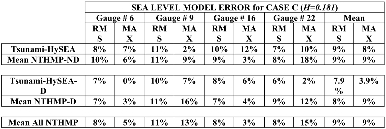
Table BP6.1.c Sea level time series Tsunami-HySEA model error with respect to laboratory experiment data for Case C (H=0.181). Comparison with the mean value obtained for the 8 models performing this benchmark in NTHMP (2012) separated among non-dispersive (Alaska, Geoclaw, and MOST) and dispersive models (ATFM, BOSZ, FUNWAVE, NEOWAVE, and SELFE), for a more precise comparison. RMS: Normalized Root Mean Square Deviation Error. MAX: Maximum runup relative error. The values for NTHMP models are taken from data in Table 1-9 c
Tasks to be performed
Task 3 Runup around the island
Figure BP6.3 presents the runup numerically computed around the island with the non-dispersive model, compared against the experimental data for the three cases. Figure BP6.3D shows the same comparison but for the dispersive model. The values for the NRMSD and maximum error runup are computed and shown in the figures. Table BP6.2 gathers the values for these errors for Tsunami-HySEA (dispersive and non-dispersive) and compared them with the mean of the model in NTHMP (2012).
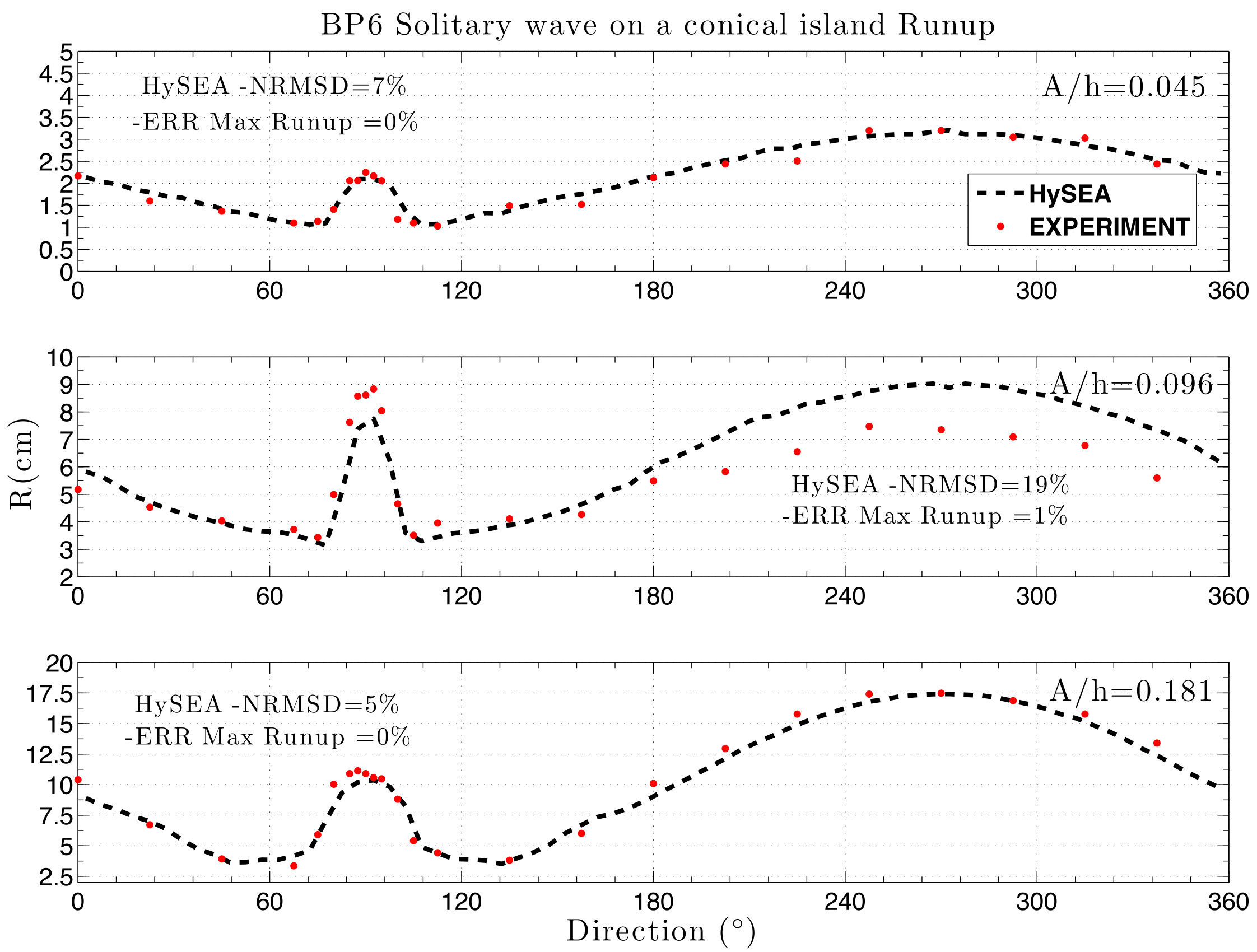
Figure BP6.3. Comparison between the computed and measured runup around the island for the three cases. Non-dispersive results.
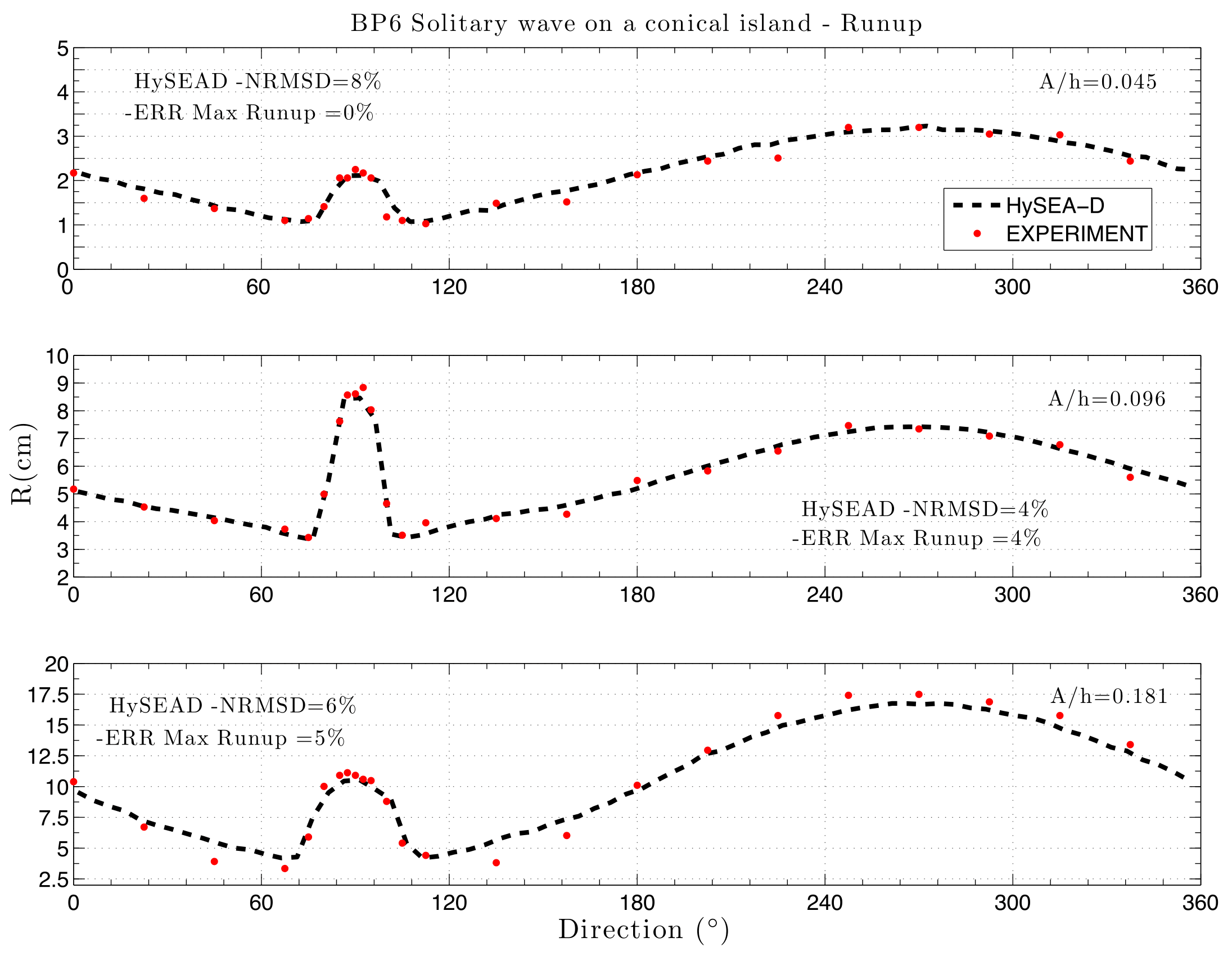
Figure BP6.3D. Comparison between the computed and measured runup around the island for the three cases. Tsunami-HySEA dispersive model.
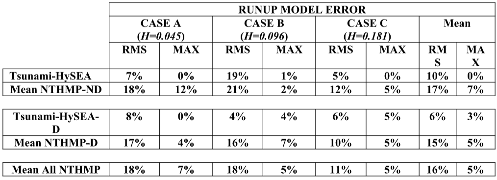
Table BP6.2. Runup Tsnami-HySEA model error with respect to laboratory experiment data for all Cases A, B, and C. Comparison with the mean value obtained for the 8 models performing this benchmark in NTHMP (2012) separated among non-dispersive (Alaska, Geoclaw, and MOST) and dispersive models (ATFM, BOSZ, FUNWAVE, NEOWAVE, and SELFE), for a more precise comparison. RMS: Normalized Root Mean Square Deviation Error. MAX: Maximum runup relative error. The values for NTHMP models are taken from data in Table 1-10