Benchmark Description
This benchmark is the lab counterpart of BP1 (analytical benchmarking comparison). In this laboratory test, the 31.73 m-long, 60.96 cm-deep and 39.97 cm-wide wave tank located at the California Institute of Technology, Pasadena was used with water of varying depths. The set of laboratory data obtained has been extensively used for many code validations. In this BP4 the data sets for the H/d=0.0185 nonbreaking and H/d=0.30 breaking solitary waves are used for code validation. The model has been firstly run in non-linear, non-dispersive mode. Then a dispersive version of Tsunami-HySEA has also been used to assess the influence of dispersive terms in both, non-breaking and breaking cases, and in both wave shape evolution and maximum runup estimation.
Problem Setup
Problem set-up is defined by the following items:
- Friction. Manning coefficient was set to 0.03 for the non-dispersive model and slightly adjusted for the dispersive model (0.036 for the H/d=0.30 and 0.032 for H/d=0.0185).
- Parameters: d=1, g=1, and H=0.0185 for the nonbreaking case and H=0.30 for the breaking case.
- Computational domain. The computational domain in x spanned from x=-10 to x= 70.
- Boundary conditions. A non-reflective boundary condition at the right side of the computational domain is imposed.
- Initial condition. The prescribed soliton at time t=0 with the proposed initial velocity.
- Grid resolution. The numerical results presented are for a computational mesh composed of 1600 cells, i.e., x=0.05=d/20.
- Time stepping. Variable time stepping based on a CFL condition.
- CFL. CFL number is set to 0.9
- Version of the code. Tsunami-HySEA third order (non-dispersive) and second order dispersive codes have been used.
Tasks to be performed
- Compare numerically calculated surface profiles at t/T=30:10:70 for the non-breaking case H/d=0.0185 with the lab data (case A);
- Compare numerically calculated surface profiles at t/T=15:5:30 for the breaking case H/d=0.3 with the lab data (case C);
- Numerically compute maximum runup (case A and C);
- Numerically compute maximum runup R/d versus H/d.
Tasks to be performed
Task 1 Water level at 30, 40, 50, 60, and 70 (d/g)^1/2 for Case A (H/d=0.0185)
Figure BP4.1 shows the numerical results for Task 1, comparing the computed and measured surface profiles for the low amplitude case (A) using the non-dispersive version of Tsunami-HySEA. Figure BP4.1D presents the same comparison but for the dispersive version of the code. Table BP4.1 gathers the values for the Normalized Root Mean Square Deviation (NRMSD) and the maximum amplitude or runup error (MAX) for this case for both non-dispersive and dispersive models and compares them with the mean of the eight models in NTHMP (2012) performing this benchmark problem. For comparison purposes models in NTHMP (2012) have also been split into dispersive (5 of them) and non-dispersive (3), and the mean values for the errors presented in Table BP4.1. Values for NTHMP models extracted or computed from data in Table 1-8 a in page 41.
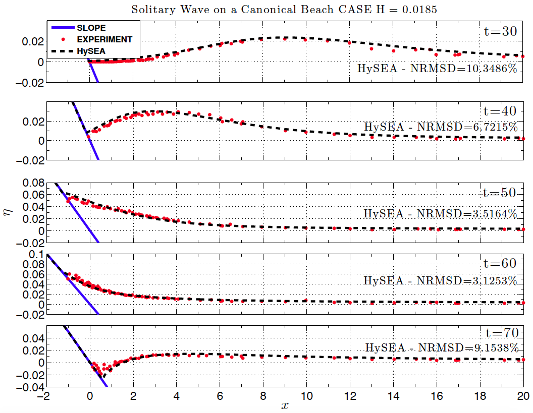
Figure BP4.1 Comparison of numerically calculated free surface profiles at various dimensionless times for the non-breaking case H/d=0.0185 with the lab data. Non-dispersive Tsunami-HySEA model.
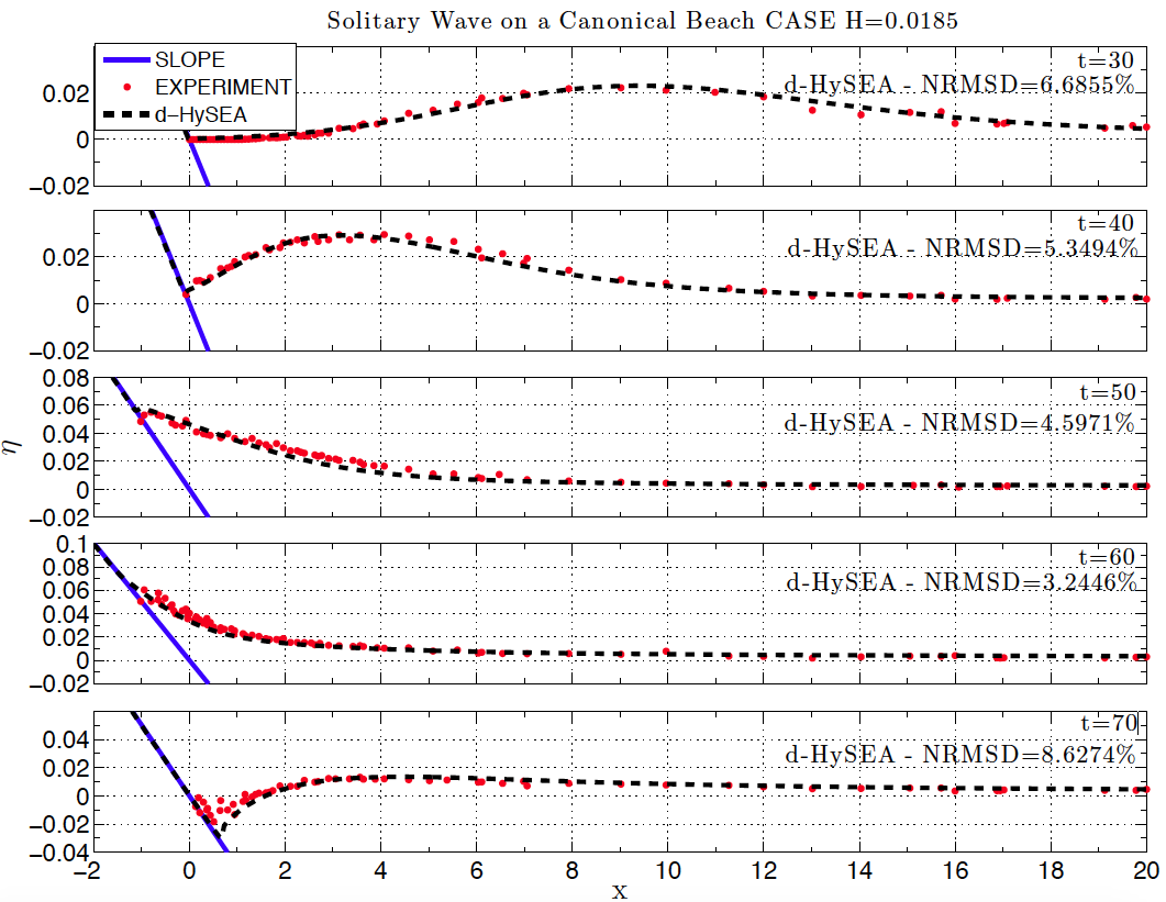
Figure BP4.1D Comparison of numerically calculated free surface profiles at various dimensionless time for the non-breaking case H/d=0.0185 with the lab data. Dispersive Tsunami-HySEA model.
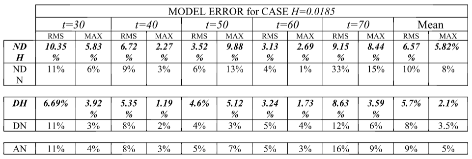
Table BP4.1. Tsunami-HySEA model surface profile errors with respect to the lab experiment for Case A, H=0.0185 at times t=30:10:70 (d/g) 1/2 . RMS: Normalized root mean square deviation, MAX: Maximum amplitude or runup error. NDH: Tsunami-HySEA non-dispersive, NDN: Non-dispersive models in NTHMP (2012) (Alaska, GeoClaw, and MOST); DH: Tsunami-HySEA dispersive; DN: Dispersive models in NTHMP (2012) (ATFM, BOSZ, FUNWAVE, NEOWAVE, and SELFE); AN: Mean of all models in NTHMP (2012). The values for NTHMP models are taken or computed from data in Table 1-8 a in page 41 of the NTHMP report.
Tasks to be performed
Task 2. Water level at 10, 15, 20, 25, and 30 (d/g) 1/2 for Case C (H/d=0.3)
Figure BP4.2 shows the numerical results for Task 2, comparing the computed and measured surface profiles for the high amplitude case (C) using the non-dispersive version of Tsunami- HySEA. Figure BP4.2D presents the same comparison but for the dispersive version of the code. Table BP4.2 gathers the values for the Normalized Root Mean Square Deviation (NRMSD) and the maximum amplitude or runup error (MAX) for this case for both non-dispersive and dispersive models and compares them with the mean of the four non-dispersive models in NTHMP (2012) that presented their results for this test (ATFM, BOSZ, FUNWAVE, and NEOWAVE). The models in NTHMP (2102) not including dispersive terms did not present results for this test (data extracted from Table 1-8 b in page 41).
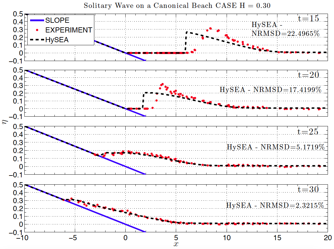
Figure BP4.2 Comparison of numerically calculated free surface profiles at various dimensionless times for the breaking case H/d=0.3 with the lab data. Non-dispersive model.
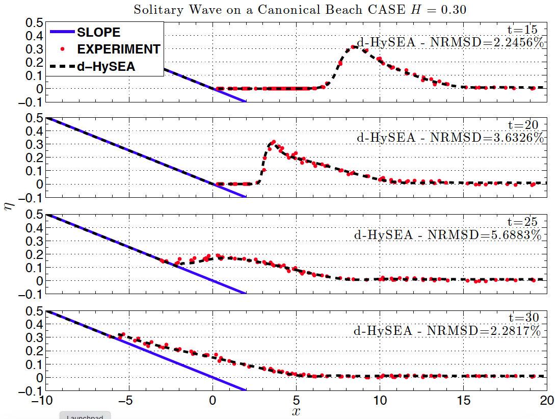
Figure BP4.2D Comparison of numerically calculated free surface profiles at various dimensionless time for the breaking case H/d=0.3 with the lab data. Dispersive model.
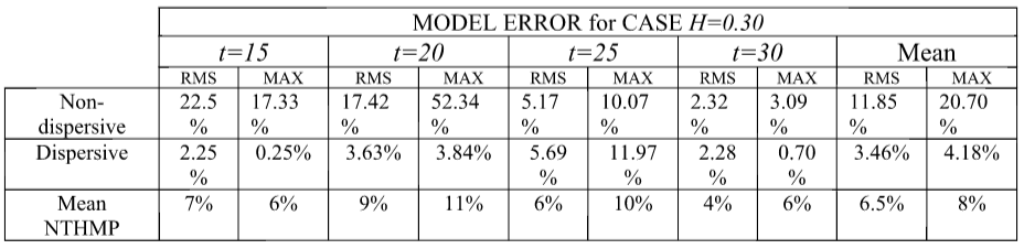
Table BP4.2. Tsunami-HySEA model surface profile errors with respect to the lab experiment for Case C, H=0.30 at times t=15:5:30 (d/g) 1/2 . RMS: Normalized root mean square deviation, MAX: Maximum amplitude or runup error. Non-dispersive, dispersive model results and the mean of the 4 models with dispersion in NTHMP (2012) that presented results for this test are collected in this table. The values for NTHMP models are taken from data in Table 1-8 b in page 41 of the NTHMP report.
Tasks to be performed
Task 3 Maximum runup (Case A and C)
Figure BP4.3 shows the maximum runup as a function of time for Case A and Case C. Numerical results for models without and with dispersion are presented for comparison in each figure. The maximum simulated runup is marked in the time series. In case (A) the maximum runup of 0.08066 is reached at time t=56-56.5 s for the non-dispersive model and at time t=56.5s for a height of 0.0802 for the dispersive model. In case (C) a maximum runup height of 0.5117 is reached at time t=42-42.5 s for the non-dispersive model and of 0.512 at t=43.5 s for the dispersive model. These values are marked with red and green dots (respectively) in Figure BP4.3.

Figure BP4.3. Maximum runup as a function of time. Upper panel Case A. Lower panel Case C. Red dots mark the maximum runup over time for non-dipersive model and green dots for the dispersive model.
Tasks to be performed
Task 4 Maximum runup R/d versus H/d
Figure BP4.4 shows the maximum runup, R/d, as a function of H/d for the numerical simulations performed without dispersion (red dots) and including dispersion (green dots). For the two numerical experiments, with H/d=0.30 and H/d=0.0185, the computed values for the maximum runup computed without and with dispersion cannot be distinguished in the graphics as the values only differ slightly. In the same figure a scatter plot of more than 40 lab experiments conducted by Y. Joseph Zhan are depicted.
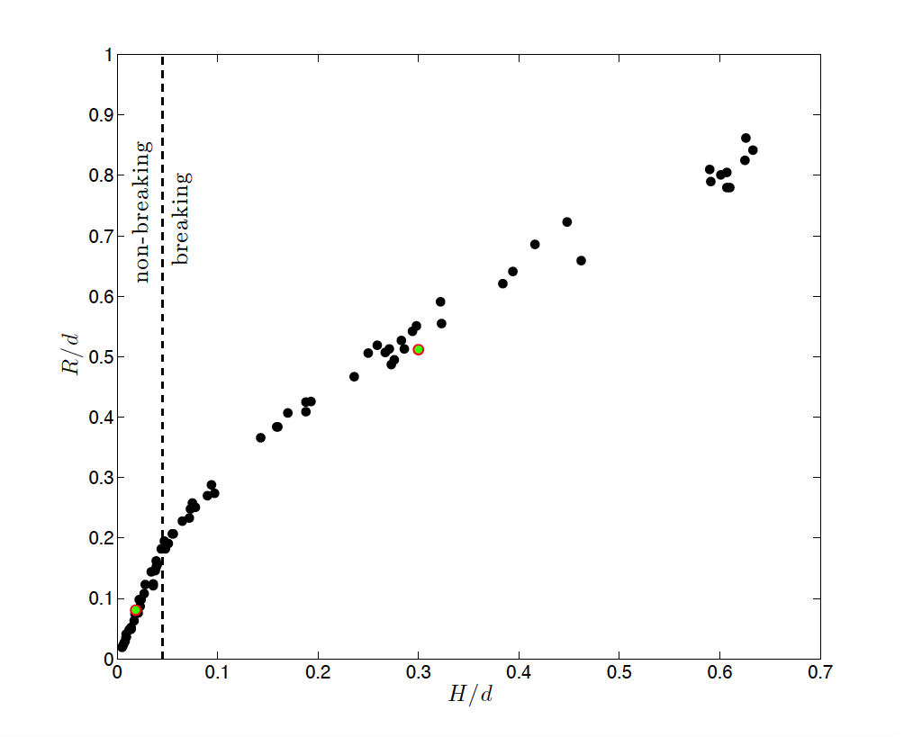
Figure BP4.4. Scatter plot of non-dimensional maximum runup, R/d, versus non-dimensional incident wave height, H/d, resulting from a total of more than 40 experiments conducted by Y. Joseph Zhan. Red dots indicate the non-dispersive numerical simulations and the green dots the results for the dispersive model. Numerically they are slightly different but in the graphic they superimpose