Benchmark Description
In this section, we compare numerical results for solitary wave shoaling on a plane beach to an analytic solution based on the shallow water equations. The benchmark data for comparison are obtained from NTHMP (2012) or Synolakis et al. (2008). In the present case, the model has been run in non-linear, non-dispersive and no friction mode as requested for comparison and verification purposes. In this problem, the wave of height H is initially centered at distance L from the beach toe and the shape for the bathymetry consists of an area of constant depth d, connected to a plane sloping beach of angle b=arccot(19.85) as schematically shown in Figure 1.
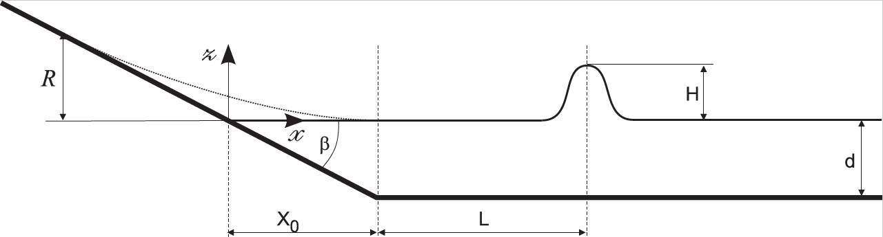
Figure 1. Non-scaled sketch of a canonical 1D simple beach with a solitary wave (X0=d cot b).
Problem Setup
Problem set-up is defined by the following items:
- Friction. No friction (as required).
- Parameters: d=1, g=1, and H=0.019.
- Computational domain. The computational domain in x spanned from x=-10 to x= 70.
- Boundary conditions. A non-reflective boundary condition at the right side of the computational domain is imposed (beach slope is located to the left).
- Initial condition. The prescribed soliton at time t=0 with the proposed correction for the initial velocity.
- Grid resolution. The numerical results presented are for a computational mesh composed of 800 cells, i.e., x=0.1=d/10. For the converge analysis of the maximum runup two other increased resolutions have been used, x=0.05=d/20 and x=0.025=d/40 with 1600 and 3200 cells, respectively.
- Time stepping. Variable time stepping based on a CFL condition is used.
- CFL. CFL number is set to 0.9
- Version of the code. Tsunami-HySEA third order is used
Tasks to be performed
- Numerically compute the maximum runup of the solitary wave.
- Compare the numerically and analytically computed water level profiles at t=25(d/g)^1/2 , t=35(d/g)^1/2 , t = 45(d/g)^1/2 , t = 55(d/g)^1/2 , and t = 65(d/g)^1/2. Note that as we used the MATLAB scripts and data provided by Juan Horrillo, the numerical vs analytical comparison is performed at the times given in the provided data and depicted by the corresponding MATLAB script, that do not correspond exactly with all the time instants given in BP1 description. More precisely, they do correspond to t=35:5:65 (d/g)^1/2 . Therefore, t=25(d/g)^1/2 is missing and t=40, 50, and 60(d/g)^1/2 are shown.
- Compare the numerically and analytically computed water level dynamics at locations x/d=0.25 and x/d=9.95 during propagation and reflection of the wave.
- Demonstrate scalability of the code.
Tasks to be performed
Task 1. Maximum runup
The maximum runup is reached at t=55(d/g)^1/2 . In the case of the reference numerical experiment with x=0.1 and 800 cells the value for the maximum runup is 0.08724. For the refined mesh experiments with x=0.05 and x=0.025, the computed runup are 0.09102 and 0.9165, respectively. Comparison of the numerical solutions with the analytical reference is depicted in Fig. BP1.1, showing the convergence of the maximum runup to the analytical value as mesh size is reduced. It must be noted, that for the analytical solution at time t=55(d/g)^1/2 and location x=- 1.8 water surface is located at 0.0909, but this in not the value of the analytical runup (that must be a value slightly above 0.92), as can be seen in Fig. BP1.1.
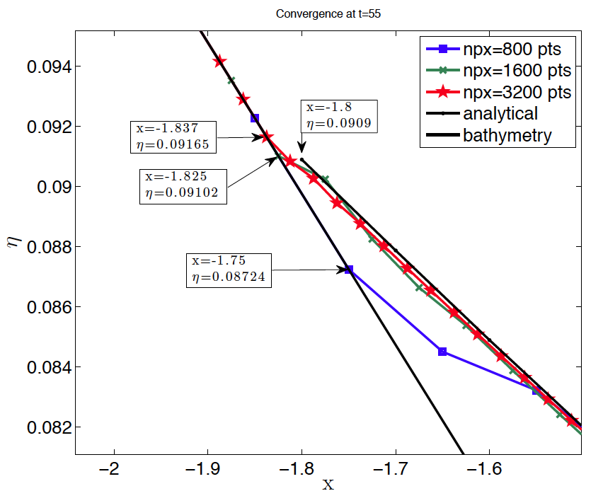
Figure BP1.1 Water level profiles during run-up of the non-breaking wave in the case H/d = 0.019 at time t=55(d/g)^1/2 for three different numerical resolutions. Comparison with the analytical solution.
Figure BP1.2 depicts the time evolution for the maximum runup simulated for the three spatial resolutions considered. The black dot marks the approximate location of the analytical maximum runup.
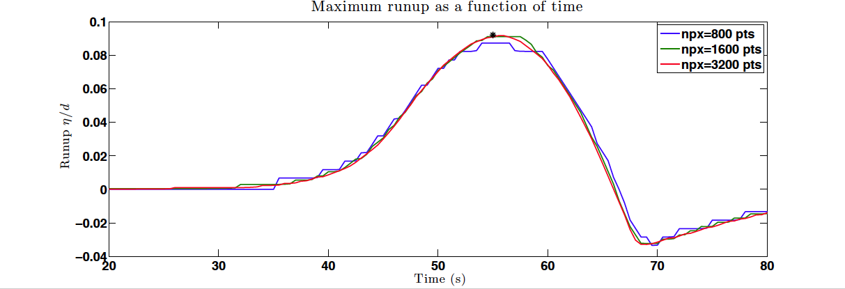
Figure BP1.2 Maximum runup as a function of time for the three resolutions considered. The black dot showing the analytical maximum runup at t=55 s.
Tasks to be performed
Task 2. Water level at t=35:5:65 (d/g) 1/2 . (MATLAB script and data from J. Horrillo).
The next two figures show the water level profiles during the run-up of the non-breaking wave in the case H/d=0.019 on the 1:19.85 beach at times t=35:5:50 (d/g)^1/2 in Fig. BP1.3.a and times t=55:5:65 (d/g)^1/2 in Fig. BP1.3.b. For comparison with the analytical solution Normalized. Root Mean Square Deviation (NMRSD) and Maximum Wave Amplitude Error (ERR) are computed and shown for every time.
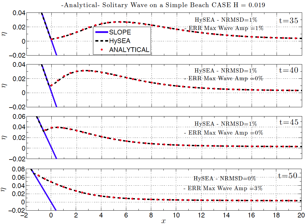
Figure BP1.3.a Water level profiles during run-up of the non-breaking wave in the case H/d = 0.019 on the 1:19.85 beach (at times t=35(d/g)^1/2 , t=40(d/g)^1/2 , t = 45(d/g)^1/2 , and t = 50(d/g)^1/2 ).
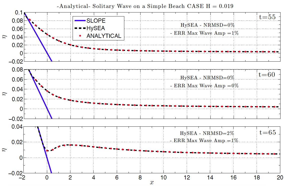
Figure BP1.3.b Water level profiles during run-up of the non-breaking wave in the case H/d = 0.019 on the 1:19.85 beach (at times t=55(d/g)^1/2 , t=60(d/g)^1/2 , and t = 65(d/g)^1/2 ). NRMS: Normalized root mean square deviation, MAX: Maximum amplitude or runup error.
Table BP1.1 presents the values that measure model surface profile errors with respect to the analytical solution for H=0.019 at considered times. The error value for a particular time is rounded towards the nearest integer. The mean values are computed exactly, using the exact values for all times. Mean values for the eight models in NTHMP (2012) report are presented for comparison (taken from Table 1-7 a, in page 38, of NTHMP (2012)).
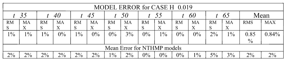
Table BP1.1. Tsunami-HySEA model surface profile errors with respect to the analytical solution for H=0.019 at times t=35:5:65 (d/g)^1/2 . RMS: Normalized root mean square deviation, MAX: Maximum amplitude or runup error. Comparison with the mean value for NTHMP models in NTHMP (2012).
Tasks to be performed
Task 3 Water level at locations x/d=0.25 and x/d=9.95
Figure BP1.4 depicts the comparison of the water level time series of numerical results at both locations, x/d=0.25 and x/d=9.95, with the analytical solution. Table BP1.2 collects the values that measure model sea level time series errors with respect to the analytical solution for H=0.019 at locations x=9.95 and x=0.25. The error value for each location is rounded towards the nearest integer. Mean values for Tsunami-HySEA are computed exactly.

Figure BP1.4. Water level time series at location x/d = 9.95 (upper panel) and at location x/d = 0.25 (lower panel). Mesh resolution 800 points.

Table BP1.2. Tsunami-HySEA model sea level time series errors with respect to the analytical solution for H=0.019 at x=9.95 and x=0.25. RMS: Normalized root mean square deviation, MAX: Maximum amplitude or runup error. Comparison with the mean value for NTHMP models in NTHMP (2012), taken from Table 1-7 b in page 38 of NTHMP report.
Tasks to be performed
Task 4. Scalability
Tsunami-HySEA has the option of solving dimensionless problems, and this is an option commonly used. When dimensionless problems are solved, it makes no sense to perform any test of scalability as the dimensionless problems to be solved for the different scaled problems will (if scaled to unity) always be the same one.